Time versus rate
Encoding (and decoding) with spikes
Last lecture, we saw how spikes are generated from a fluctuating membrane potential. But why do neurons send discrete spikes instead of continuous voltage? Over long distances, physics tells us that voltage decays exponentially. To maintain the signal, it must be amplified as it travels down the axon. The solution is to send strong signals in the form of action potentials, i.e. spikes.
There are two primary ways to convey information through spikes: a time code and a rate code. Which is the brain using? This is one of the oldest debates in neuroscience, and when you have very informed people on either extreme, the answer is usually somewhere in between, or both. In this post, we’ll take a whirlwind tour through evidence for both sides, and also talk about oscillations (which are… kind of both).
Last time, we described the deterministic leaky integrate-and-fire (LIF) neuron. Although you could still measure a firing rate of such a neuron, information is conveyed in the precise timing of the spikes. Said another way, the LIF would have exactly the same output across different trials of the same experiment. In contrast, the linear-nonlinear Poisson neuron (LNP) generates spikes through a random Poisson process, with nondeterministic timing. Information is conveyed, by design, through the spike rate. For the LNP, different trials would all look different, but their spike rates on average would be about the same. Of course, these neuron models each have various caveats, but we use them to illustrate the opposing regimes.
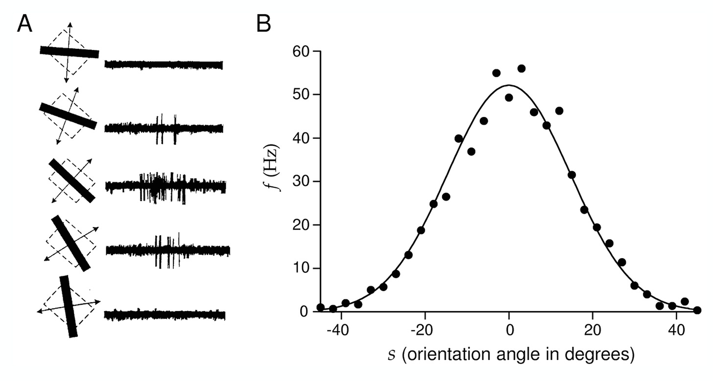
In physiology, the classic example of single cell recordings comes from the 1960s experiments of David Hubel and Torsten Wiesel in cat primary visual cortex. Neurons are tuned to orientations of bars (A), meaning that there is a tuning curve (B) of firing rate as a function of orientation angle. This supports the rate coding hypothesis. It looks random: if you did this trial again, there would be a different set of spike times with the same firing rate on average.

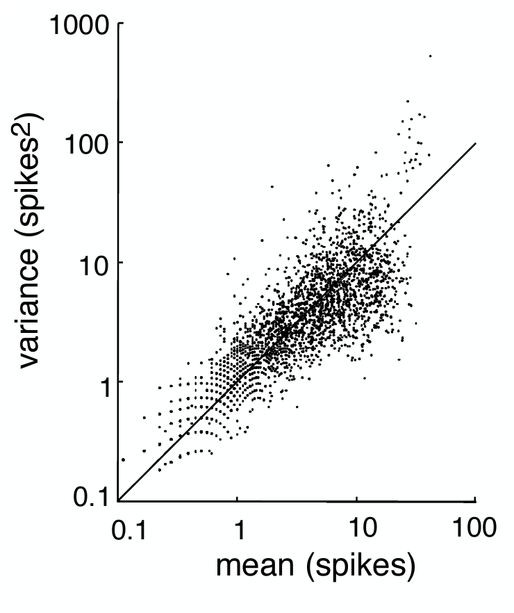
An implication of the rate coding hypothesis is that there must be noise in the system, shown here by the data points deviating from the fitted curve at higher firing rates. If we model spikes with a Poisson process, the variance should be equal to the mean. Lo and behold, in the middle temporal visual area of macaque monkeys shown movie stimuli, this was found to be roughly empirically true.

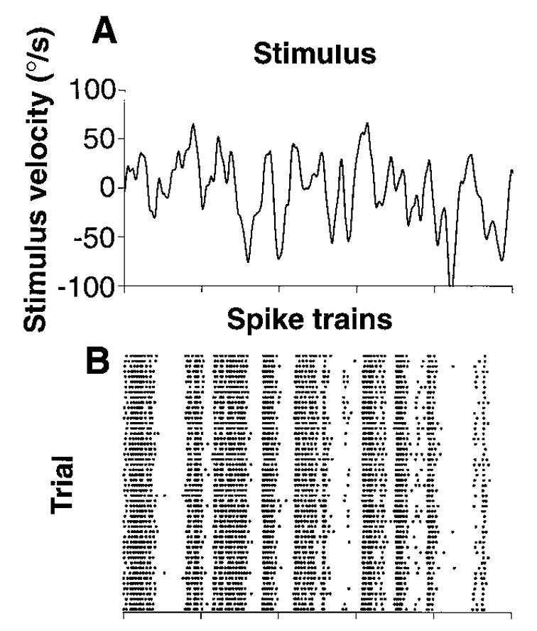
In the fly H1 neuron, which responds to horizontal motion, this Poisson relationship was also found in response to a stimulus of constant velocity. However, what if we have a stimulus that varies velocity across time? Suddenly, the the relationship is no longer Poisson. The spike patterns appear to be timed with specific changes in stimulus velocity or direction. This is not a rate code.

In a rat cortical neuron, spike timing response to an injected constant current (left) appears to become noisier as time goes on. The firing rate seems about the same, but the timing looks random. But when a time-varying signal is injected, the spike timing is synchronized to fluctuations in the signal (right). Unlike the time-varying signal, the constant signal gives nothing for the neurons to synchronize with, so their fluctuations in timing are due to other processes.

The results from this experiment should make you uncomfortable, Bruno says. When people saw these results, it certainly had that effect. There were mixed reactions: some people took the left response as confirmation that spiking is governed by a random process under some regimes. Others took it as evidence that spike timing is deterministic when there is signal driving it, and that the seemingly random responses are a result of other processes in the neuron not quantified by us. We don’t have access to the state of the neuron, and we can’t observe all the variables that generate spikes.
Based on studies like these, the answer to the time vs. rate question is unsatisfying. Sometimes, things appear to be random. And sometimes, they appear to be deterministic. We probably need to look at both the timing and the rate?
Here’s an example of this. The nerve fibers in the auditory system seem to be phase-locked, which kind of codes both timing and rate simultaneously: the neurons fire at a specific position in a cycle of the incoming signal (hair cells wiggling). Each row below shows a histogram over many trials of the spikes from an auditory nerve fiber. The rows are ordered by the frequency the fiber is the most sensitive to, determined by the corresponding position on the basilar membrane1. The punchline here is that each nerve fiber fires when there is energy in the signal at its characteristic frequency, but the timing of the spike also reflects the signal frequency!

In addition to the oscillations, the frequency information is transmitted two ways: in the tonotopic code (where the neuron is on the basilar membrane tells you the frequency), and in the phase-locked spike times. Because the tuning of the cells — the frequency they are most sensitive to — is relatively broad, there is some ambiguity to the tonotopic code. A cell could fire in response to 500 Hz, but it could also fire to 510 Hz. The exact timing of the spikes gives much more precision. Downstream processes can then take advantage of either, or both of these coding strategies.
This is not the only place we see oscillations. In the lateral geniculate nucleus (LGN), which sits between the eye and visual cortex in the visual processing stream, intracellular recordings reveal spikes from retinal ganglion cells. The retina was found previously to generate its own oscillations, separate from external signals2. The spikes in A below appear to be noisy, but the authors hypothesized that it was because the stimuli were out of phase with the retinal rhythm. To test this, they shifted all trials to be aligned in phase with the retinal oscillations (B). The spike timings became very precise, and what’s more, they found that there was more information encoded when looking at the timing as opposed to just the rate. Knowing the underlying process behind this initial apparent “noise” revealed that it was not noise after all.
Okay, I’ve just rambled on about a zoo of spike encoding schemes. But how do we determine how much information is actually contained in these spikes? A schematic of the decoding process is shown below, where a signal s(t) is encoded into spikes ρ(t), and then decoded into a reconstruction of the signal ŝ(t).

This is generally a hard problem, because we are trying to reconstruct a smooth, continuous signal from discrete events. The encoder is highly nonlinear, as we saw in the last post, but using a linear decoder is actually a non-absurd assumption3. It turns out that by convolving a kernel with a set of spikes, you can arrive at an approximate reconstruction. Below, we get “on” and “off” spikes via a LIF neuron on the signal and the sign-reversed signal. Then, we convolve the on spikes with the kernel, and the off spikes with the negative kernel. You could also do this with only on spikes and a different kernel.
By showing this decoding procedure, we are not implying that the brain literally reconstructs the signal somewhere downstream of the spikes. This is just one way of quantifying the information contained in the spikes that can be utilized in subsequent processes.
We can also do this using information theory. I won’t go into detail here4, but the remarkable thing about this analysis, applied across many systems and organisms, is that you sometimes get on the order of 2-3 bits of information per spike, rather than just 1 bit, as you’d expect from a binary signal. How? The key is that when the neuron is not spiking, there is also information conveyed; it’s the pattern of spikes over time that matters.
Personally, it’s obvious after seeing all these examples that there is no single answer to the timing vs. rate debate; there is clearly a diverse set of coding schemes dependent on the type of computation being performed. Putting this aside for now, the next lecture will get into coding more abstractly with one example: what is the most efficient way to encode natural scenes based on their statistics, and how does the retina do it?
Long-range synchronization of oscillatory light responses in the cat retina and lateral geniculate nucleus, Neuenschwander & Singer (1998). This was a controversial paper, and it took decades for people to reproduce the findings and believe it.
You can see motivation for this assumption in the joint distribution of spikes and signals: the decoding marginal distribution is roughly linear in number of spikes.


