Stable states
A brief introduction to attractor networks in theoretical neuroscience

In October, John Hopfield and Geoffrey Hinton won the Nobel Prize in Physics for “foundational discoveries and inventions that enable machine learning with artificial neural networks”. Hopfield was recognized for his theoretical model of associative memory based on the Ising model from physics, and Hinton for a generative, probabilistic neural network1. Though there is no doubt both scientists have contributed significantly to their respective fields, the decision seems to imply that physics-based models like the Hopfield Network and Restricted Boltzmann machine have heavily influenced current ML/AI. This is not true, to my knowledge (if you believe otherwise, I’d like to hear it)2. A different take is, of course:
That said, Nobel Prizes and this weird worship of single scientists doesn’t make much sense to me. Science is only possible through collaboration and building off others’ work3, not to mention all the other factors that allow us to be in the privileged position of doing science in the first place.
Regardless of their relationship to AI, we can learn a lot from these elegant models. Attractor networks (this post) and probabilistic models (next post) are central to theoretical neuroscience.
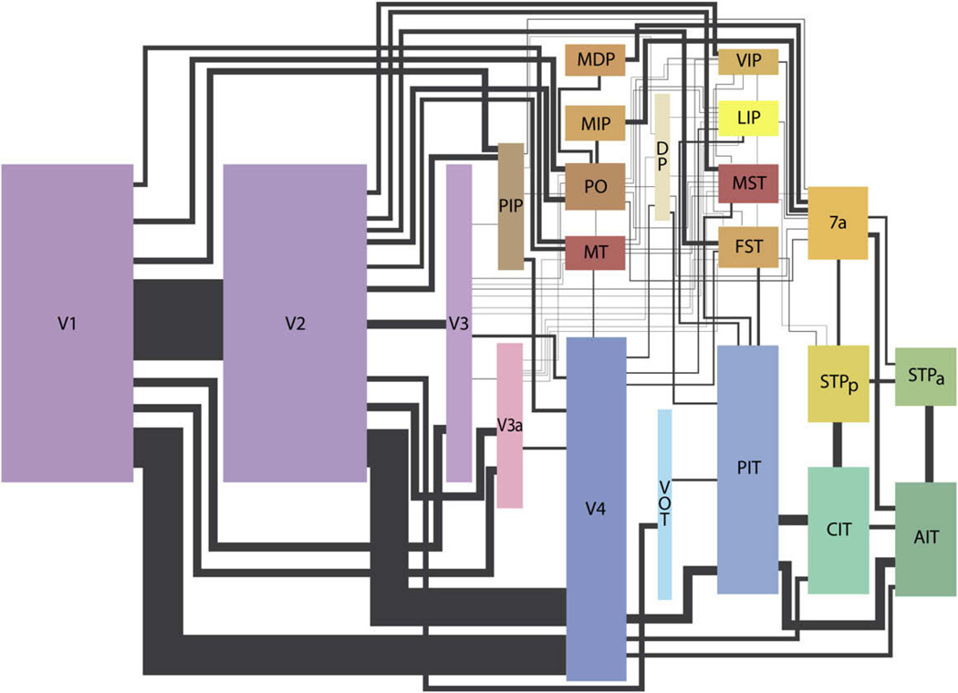
The brain is highly recurrent. We saw this diagram of cortex and its wirings in a previous lecture:

The connections between cortical areas, represented by the lines, go in both directions. Complex dynamics govern the recurrent interactions between brain areas. In 1982, Hopfield brought ideas from statistical physics as a starting point to model these relationships.
Given a dynamical system, which is a set of variables that change over time according to some equations, we can analyze its state, or the setting of its variables at a moment in time. An attractor network is a dynamical system whose variables converge to a particular state (or a set of states, as we will see later) as time goes on.
The Hopfield Network
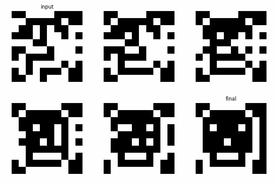
An associative memory is a system that takes content as input (as opposed to a memory address), e.g. image pixels, and retrieves the most likely match from stored memories. The Hopfield Network is a recurrent dynamical system that returns a stored pattern given some input pattern that could be noisy or incomplete. The below example shows a noisy binary input and running the dynamics until the correct pattern is recalled.
Implementing an associative or content-addressable memory is a hard problem as the number of patterns increases, but humans are able to robustly recall patterns in this way. For example, if you hear a snippet of a song you know, even if it’s in a noisy environment or a bad karaoke, you can sing the part that follows without much effort. While we do not know how the brain does it, we start by analyzing a simple recurrent system.
The basic Hopfield Network consists of a set of units V that take on values of either -1 or 1. They have all-to-all connections in both directions defined by symmetric weight matrix T, which is where the patterns are stored.
To store, we follow the weight update rule
where α indexes the patterns. For each pattern, this forms a basin of attraction that the values are pushed toward. Note that we store multiple patterns in one weight matrix by simply adding the unit value products (superposition).
Given a set of weights where patterns have already been stored and some initial unit values (input), we select a unit and update its values according to the rules
We then move on to another unit, and repeat until convergence, i.e. when the values stop changing. At this point, we have recovered the stored pattern that is the most similar to the input. But wait, you might think (as I did initially), with these equations, couldn’t the units just flip their values back and forth forever without converging? It turns out the answer is no.
To the system of neurons, we can assign an energy, which we would like to minimize over time. We can prove that Hopfield Network dynamics will always maintain or decrease the energy, and converge to a stable, low-energy fixed point4. Intuitively, we know this energy will be lowest when the product of unit values matches the connection between them. Since the memories are stored in the weights, the units will change values until they all correspond with the weights as well as possible.
Although the dynamics are guaranteed to converge, they are not guaranteed to retrieve the correct pattern because of the way memories are stored. Each network has a capacity for how many memories it can recall accurately, which is ~0.14N where N is the number of neurons in the network. If the patterns are very similar, then this number becomes even smaller. Bruno has a nice handout on attractor networks that goes much more in-depth than I do here, and there are tons of comprehensive tutorials on Hopfield Networks out there, e.g. Bhiksha Raj’s lecture, that can help give more intuition to how these dynamics work.
In the context of neuroscience, an obvious question arises: does the Hopfield Network map onto an actual mechanism in the brain? Not that I know of, but it’s a nice starting point for learning about recurrent neural models. As for the AI side, there are some connections between Hopfield Networks and current machine learning algorithms, such as the attention mechanism in transformers (which are behind LLMs) via the modified Modern Hopfield Network5. But as far as I know, this post-hoc connection was formulated after the success of transformers, and the Hopfield Network has not really played a part in current AI.
A ring attractor for head direction
Here’s an example of an attractor network that we can relate more concretely to a real biological mechanism. Rats have cells that are selective to a specific head direction (an angle from 0 to 360) with respect to some external reference point.

In 1996, Kechen Zhang proposed a ring attractor circuit and dynamics to simulate this head direction-tuned cell activity. Others had previously suggested similar circuits (e.g. Skaggs 1995), but Zhang concretized it with math.
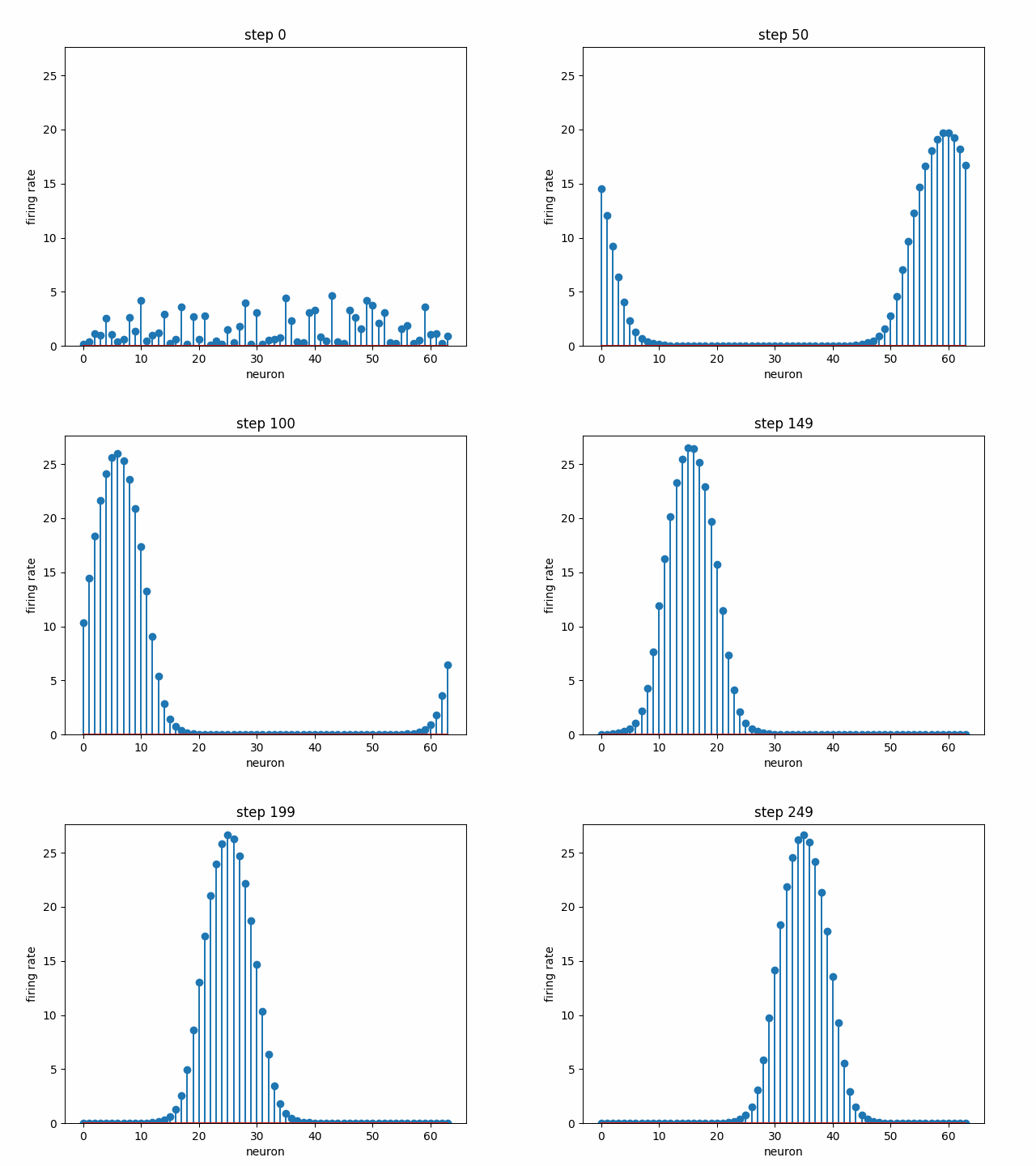
Given a set of neurons, each with a different preferred head direction θ₀ (i.e. each one has a peak like in the above plot, but at a different angle), how can we connect them with some weights and dynamics such that there is a stable “bump” in neural activity that encodes head direction? In the below simulation, 64 neurons are each initialized to some random firing rate. Over time, the dynamics cause convergence to a stable bump, where the peak indicates the neurons that are the most selective to the current head direction. Note that this not the same bump as the above plot; we are modeling the population dynamics of recurrently-connected neurons, not the tuning of a single neuron.
Contrasting with the point attractor dynamics in the Hopfield Network, a ring attractor allows us not only to have multiple stable points of attraction, but also gives us a way to move smoothly between them. Because we are modeling an angular variable, head direction, it is natural to use a ring topology (once we hit the end, we return to the beginning). What if the rat is turning in space? We would like the movement of the bump to reflect this, i.e. shifting the bump corresponds to the rat’s rotation. Below is the model population activity as the rat is turning at a constant velocity in one direction. Despite shifting position, the bump maintains its shape.
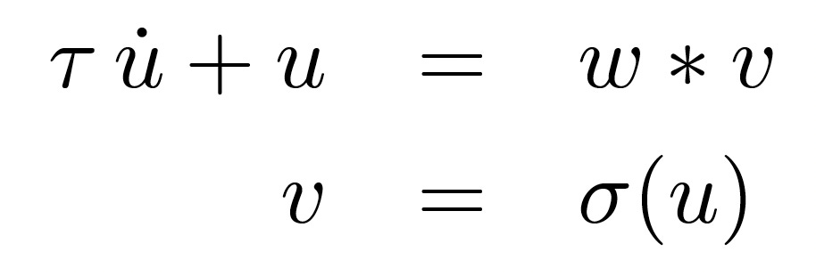
The dynamics for the stable bump are quite straightforward. Below, u is a vector that represents the membrane potential of the units, u̇ is the population change over time, and v is a vector of firing rates, produced from a point-wise nonlinear function σ of u. ∗ indicates convolution. w is a vector of weights, which we must define to induce this stable bump structure.
It turns out the correct w looks like the below left: for one unit, we want its neighboring units to be excited, and ones far away to be inhibited. More generally, for a whole set of neurons, we get the matrix on the right, which is symmetric and structured (specifically, a Toeplitz matrix6). This structure lets us formulate the dynamics with the circular convolution above. I won’t go into the derivation of w here, but it’s all in the paper.
To shift the bump, we can take the spatial derivative of the weight vector, shown in the middle row of A below. This basically says to excite neighboring cells to the right and inhibit those to the left, and add it to the original weights. The γ determines how quickly the bump is moved. The derivative helps preserve the bump shape as it’s shifting: this causes movement within the basin of the energy landscape. In a biological circuit, these added derivatives could be inputs from the vestibular system, for example, that indicate to the circuit that the animal is changing head direction.

The head direction circuit is a beautiful example of bridging theory and experimental discoveries. Zhang and Skaggs didn’t originally propose a physical configuration of these units, only a connectivity pattern via the weights. But in 2015, Seelig & Jarayaman showed that head direction activity in the fruit fly ellipsoid body — a donut-shaped structure in the brain — is literally organized on a ring. Below, the bump of neural activity on the upper left is shown via calcium imaging; on the bottom right, the blue trace shows the actual head direction, and the red trace shows the head direction decoded from neural activity.
It’s striking that theory and biology arrived at similar solutions for the dynamics of head direction cells, hinting at some fundamental principles that govern nature.
Also not too long ago, experimental studies (e.g. Green et al. 2017) showed that the bump-shifting mechanism in fruit flies involves asymmetrical connections from different populations, which could connect to Zhang’s formulation. Zhang also notes that one could also extend the 1D dynamics to a 2D sheet; there is a lot of very exciting ongoing theoretical neuroscience work (e.g. Burak & Fiete 2009) on attractor network models of 2D grid cells.
There are clearly many exciting applications in neuroscience for attractor networks, and I regret that I’m really not able to do the topic justice in this post. But we’ll move on in the next post to probabilistic models, and touch on the Restricted Boltzmann machine.
The only one I can think of is diffusion models, which are used in all (?) current state-of-the-art AI image models.
Shun-ichi Amari was actually (one of?) the first to introduce what would be known as the Hopfield Network in 1972, though his approach is more cybernetic than physics-based. His (classy) response to the Physics Nobel Prize is here. Jürgen Schmidhuber has a rant here with more historical details. Credit assignment in science is scary!
This is a Lyapunov function, so a Hopfield Network is guaranteed to converge to a fixed point under certain assumptions (symmetric weights, asynchronous weight updates).
Paul Ivanov notes that an alternative (and better, in my opinion) name would be the Hip-Hopfield Network.


