Perception as visual inference
Bayes and natural images
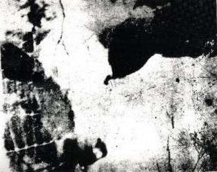
What do you see in this image?
You probably got that one, but the next one is harder. If you can’t see it, scroll to the answer at the bottom and come back!
In 1867, Hermann von Helmholtz introduced the idea of visual perception as unconscious inference: that we perceive and understand the visual world immediately and subconsciously. Illusions are interesting because our perceptual deviations from reality give us hints about the inference process. Maybe you stare at the image for a long time, and try to guess what different blobs could be. Maybe it takes knowing the answer, as is usually the case for the second image, to actually make sense of it.
Here’s another example you probably know: we see A and B as different shades, despite identical pixel values. Given the regularity of the grid and the fact that B is in the shadow of the cylinder, we infer the information that B is lighter than A. If all we were doing was processing pixel values, we would perceive A and B as the same color.

Another example is the McGurk effect, which demonstrates the interaction between vision and audition. A different video is enough to skew our perception of the consonant being spoken, even though the audio is the same. If language were only dependent on sound, they would sound identical. But our inference process depends on both sound and vision.
There are endless fun examples (e.g. see the Illusions Index), but how do we formalize perceptual inference? If we have good models of human perception, should they be fooled in similar ways by illusions1? One approach I’ll go over briefly in this post is Bayesian inference and probabilistic models.
Denoising via Bayes’ rule
This is Bayes’ rule (sans normalization term), where H = hypothesis and D = data.
It says that the posterior, the probability of your hypothesis about the world being true given the data you receive, is proportional to the likelihood, the probability that you see the data given your hypothesis, multiplied by your prior knowledge about what the hypothesis could be. There are tons of tutorials online explaining Bayes’ rule (and here’s a more detailed handout by Bruno on Bayes and generative modeling), so I’ll just go through an example application that also relates nicely to natural images statistics: removing noise from an image.
It had been common practice in the television industry to perform coring: noise reduction by removing high-amplitude, high-frequency components from a signal. Previously, this operation was a bit ad-hoc, but Simoncelli & Adelson 1996 showed how to calculate the optimal coring function for a signal using a Bayesian derivation.
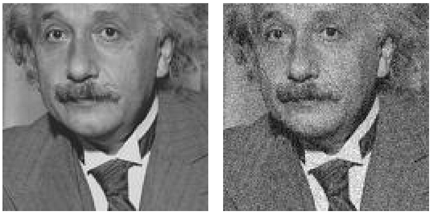
Given a simple formulation y = x + n where y is the given noisy signal, x is the clean signal, and n is some Gaussian noise, they wish to recover x̂ , an estimation of x. For example, these clean and noisy images.
Rather than taking x to be the raw pixel values of the image, they perform a 2D steerable pyramid wavelet transform on the image. If you convolve an image with an oriented, bandpass filter, you get a set of coefficients that express roughly the presence/strength of that feature present throughout the image. Doing this with a whole set of filters with different scales and orientations gets you a bunch of coefficients that serve as a summary of the image. In this paper, x, x̂ , and y refer to the coefficients from this transform, not the image pixels. For each filter, they get a distribution of coefficients that looks like the ones below.

We know that natural images do not follow a Gaussian distribution; they look like the left one, with most coefficients at or close to 0 (sparse) and with tails decaying more slowly (high kurtosis) than a Gaussian2. Given this prior knowledge about the images, and assuming that the noise is Gaussian, they want to find a way to go from a distribution with a shape like this
to the original left histogram. In Bayesian terms, they would like an estimator that has a high probability of producing the clean signal x given the noisy signal y. Suppose they want to minimize the mean squared error of the cleaned up image. Then,
which requires P(x|y), which can be calculated via Bayes’ rule:
All that’s needed is P(y|x), which is just P(n) = Normal(0, σₙ) (due to n = y - x), and P(x), which they approximate with P(y).
If one assumes the signal and noise are iid Gaussian with mean 0 and variances σₛ and σₙ, the closed form solution corresponds to a Wiener filter. But since natural images have a peakier distribution, they instead use the Laplacian distribution, and use the noisy image to estimate the distribution parameters for the clean image. See the paper for details, but on a high level, they derive an optimization problem to get coefficients x̂ for each wavelet, then convert back into the cleaned image in pixel space.
The optimal estimator they get out looks like the curvy line below:

Reading out the vertical axis, the coring function pushes small y values down and keeps larger ones approximately the same. It’s called a coring function because you can imagine roughly removing (setting to zero) the “core” (values close to zero), and it induces a distribution more peaked at 0, as desired. Applying it to the noisy image coefficients gets you the estimation of the clean image coefficients. This Bayesian approach shows a nice way to use the statistics of natural images and an assumed noise distribution to clean up an image.
Probabilistic formulation of sparse coding
Here’s another application of Bayes’ rule, applied this time to sparse coding, which I introduced briefly in a previous post. It turns out you can formulate the standard sparse coding energy function probabilistically3. Let’s just focus on the inference step, i.e. determining the sparse coefficients for an image given a dictionary (set of filters). It’s equivalent to finding the most probable configuration of coefficients a given some images I and dictionary Φ. We write the posterior probability using Bayes’ rule, in black:
In practice, we formulate inference as a minimization of the negative log probability, which results in the red equation. The first term |I-Φa|² comes from taking the log of P(I|a; Φ), for which we assume a Gaussian distribution; it’s high if the reconstructed image is different from the actual image, corresponding to the (negative) probability of whether the image I was generated from the given a (remember that sparse coding is a generative model). The second term is the prior P(a), assumed to be sparse based on our knowledge of natural image statistics (e.g. left histogram above). The sum over C(aᵢ) corresponds to the sparse image prior, where C() induces sparsity in a (assumed to be independent) and is chosen to be something like the absolute value or the Cauchy distribution. The standard method of solving is to use maximum a priori (MAP) estimation, which simply takes the mode of the posterior distribution4. I apologize for the whirlwindy explanation, but more details can be found in Olshausen & Field 1997. And if you want more details on perception as inference in general, Bruno wrote a book chapter5.
Okay, I lied last time when I said this post would cover the Restricted Boltzmann machine. I got too wrapped up in sparsity… the next post will cover RBM!
The first image in this post is a Mooney face. The second is a cow that’s often used as an example of “top-down” information influencing perception.
I won’t go over this here, but there has been decades of work on trying to model perceptual illusions, e.g. illusory contours. AFAIK there have not been clear breakthroughs yet. Current state-of-the-art models are clearly not there; Tomer Ullman recently did an investigation of illusions in LLMs.
For a review on natural image statistics see Simoncelli & Olshausen 2001.
Apparently Peter Dayan helped inspire this approach, as well as the realization that independent component analysis is a special case of sparse coding; details here.
A better way to do this is to sample from the entire posterior distribution. Fang et al. 2022 use Langevin dynamics.


