Ambient spaces

Learning manifolds

Carlsson et al. 2008.

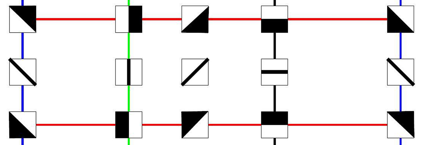
In the below cartoon, s and t are 2D points, each representing an image containing A. The most natural transformation between these two As is horizontal translation, where the midpoint between the two should correspond to an A in the middle (top point). If we were to simply linearly interpolate between the pixels of s and t, it would look like the bottom image, a superposition of two As, which is not a valid shift. The red line is the manifold of As shifted along the center horizontal axis of the image. Possible points can lie anywhere in 2D, but all possible horizontal translations lie on a (specific) line, which is 1D. Note also that the position of the point on the red line also tells you the horizontal position: it explicitly parameterizes amount of shift.

Formally, a manifold is a topological space that is locally approximately Euclidean. As I am not a mathematician, I hope you’ll forgive me (and many others) for using manifold here more as a conceptual device (with selected mathematical tools) to help reason about the geometry of data that lie on some high-dimensional space. In 2D, manifolds include lines and circles (1D structures embedded in 2D space), and in 3D, surfaces such as planes, spheres, and toruses (2D structures embedded in 3D space).

What about real data? If you had a set of natural images each of size p pixels, the manifold of natural images would be n-dimensional, where n < p. That is, if you randomly selected p values for an image, this would probably look like noise, and would unlikely fall on the n-dimensional natural image manifold. “Walking” on this manifold would result in natural images undergoing transformations you would expect to see in the real world, such as local translation. Fun fact: Carlsson et al. 2008 showed that the distribution of 3x3 natural image patches parameterized by oriented edges forms a 2D Klein bottle manifold.

Going back to a toy example, shown below is the classic Swiss roll problem, where the manifold is a 2D sheet rolled up in 3D. It’s not immediately clear how you would “unroll” this manifold into a flat 2D sheet. Roweis & Saul 2000 developed local linear embeddings (LLE)¹, an algorithm that finds weights to approximate each point as a linear combination of its local nearest neighbors (i.e. in 3D), and then uses those weights to define neighboring relationships in a new low-dimensional (i.e. 2D) space.

A. The ground truth manifold. Colors are just for visualization purposes and represent distances from one end of the sheet, but there are no values assigned to each point. B. Points are sampled from the sheet. C. After applying LLE, the points are mapped into 2D, with the points in correct order based on color. Roweis & Saul 2000.

While this algorithm unrolls the Swiss roll correctly, we are missing something crucial that the learned weights or final 2D representation don’t tell us: the structure of the original manifold. How might we learn this?

None of the representations we’ve discussed so far in the course, e.g. PCA, winner-take-all, or sparse coding, can capture manifold structure. In standard sparse coding, if you perform inference on frames of a movie, the coefficients at each frame are sparse as intended, but they change extremely quickly and incoherently. They do not reflect the persistence of features or smoothness of motion in the video. Suppose we had an object translating smoothy through space in a video; ideally, the corresponding sparse code should reflect this motion. Similar to the 2D case in the first figure, we would like our representation (sparse code) to parameterize something we care about, such as local position of some feature in the movie.

Inspired by Locally Linear Landmarks from Vladymyrov & Carreira-Perpiñán 2013, Chen, Paiton, & Olshausen 2018 developed the Sparse Manifold Transform, which performs sparse coding of high-dimensional points (resulting in localized features), and then learns a linear projection that induces flatness on a low-dimensional manifold.

The Sparse Manifold Transform. A) A function defined on 2D spatial coordinates (e.g. grayscale mages) in black; a local reconstructed component from sparse coding in red. B) Sparse coding results in a learned dictionary Φ and sparse vector α. C) Each dictionary element (black arrows) represents a landmark on some smooth manifold. Red arrows represent true underlying function, which are not in the dictionary. D) The true image component in red can be reconstructed from a linear interpolation of dictionary elements.

I’ll leave the details for another time², but this is a start in trying to learn and understand manifold structure, rather than just a mapping.

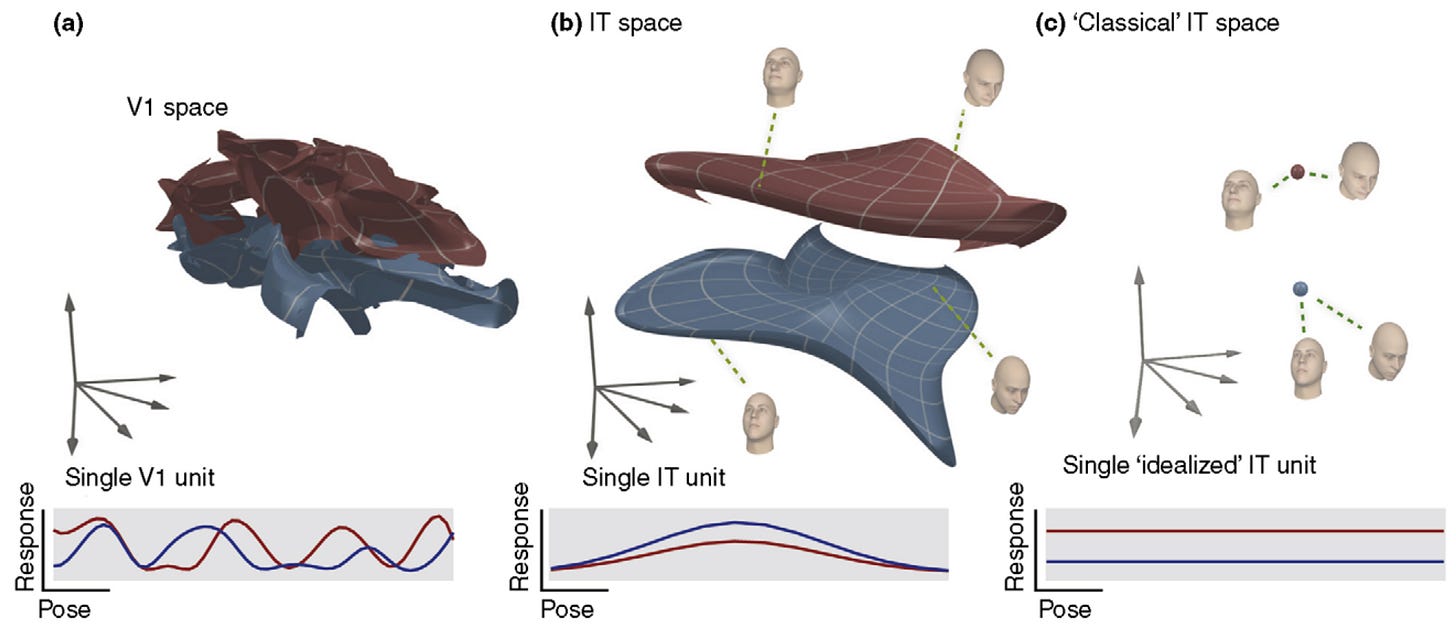
Apart from images, you could also consider manifolds in neural data space. DiCarlo & Cox 2007 proposed that the brain might perform visual object recognition by disentangling manifolds: each object has its own manifold in neural activity space, where movement along the manifold represents different transformations that the object undergoes, such as viewing angle, illumination, etc. The theory is that in early visual cortex, the manifolds are entangled and not separable; in later stages of the pathway, they become disentangled and neurons have explicit representations of object identity.

Schematic of disentangling face identity manifolds. Stimuli are two different faces shown under a variety of transformations. (a) In primary visual cortex (V1), we imagine two high-dimensional manifolds corresponding to two face identities. From a single V1 cell (real data), the response to the two faces is non-separable. (b) In inferotemporal cortex (IT) later in the ventral stream, the activity is more separable and identity is easier to decode (real data). (c) In an idealized IT unit, the two responses would be perfectly separable.

Though the term manifold is somewhat of a buzzword right now in neuroscience³ and ML, it’s a nice idea. But as far as I know, we don’t currently have specific theories for how the brain does this disentangling.

This post wraps up the unsupervised learning module of the course. Next post, we will discuss attractor dynamics, which includes Hopfield networks!

1. Tenenbaum, Silva, & Langford developed the similar method Isomaps at around the same time. The two groups published their papers next to each other in Science in 2000, along with commentary.

2. Here’s a talk by Bruno on SMT.

3. Source.